2. Simple building model

In the first example a simplified building model is connected to an ambient model which supplies the building model with the climate data of a given location (Berlin, Germany). Here you will find the explanations for several fundamental working steps for the application of the BuildingSystems library (together with Dymola 2016 or higher) such as

• the configuration of a system model structure,

• the definition of the building model parameters,

• the definition of the boundary conditions of the building model and

• the performance of a simulation experiment.

The selected building model BuildingSystems.Buildings.BuildingTemplates.Building1Zone1DBox uses a thermal 1D-modeling approach, which means all models of the building constructions (walls, roof, ground plate, etc.) are discretized regarding energy balancing in one dimension and the air space within the zone is modeled with one aggregated thermal node.

2.1. Set up the system model structure

Download the BuildingSystems library from https://github.com/UdK-VPT/BuildingSystems. Open the library with Dymola and perform the following steps:

1. Open dialog: File -> New -> Model and fill in the field Name: “SimpleBuilding”.

2. Extend the new model from Modelica.Icons.Example (see Fig. 1) and click OK.

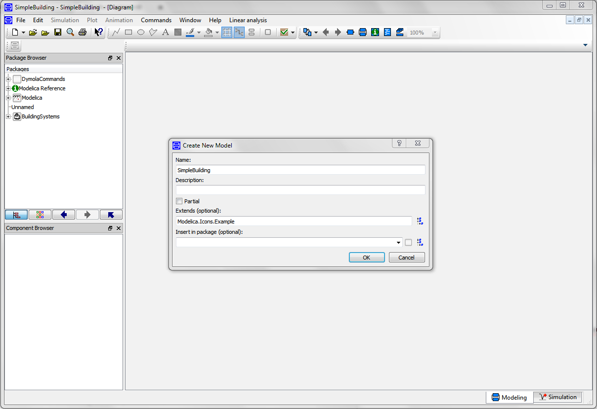
Definition of a new system model in Dymola

3. Mark the new example SimpleBuilding in the package browser and save it with File -> Save in the file SimpleBuilding.mo in a folder of your choice.

4. Ensuring that Dymola is in “Diagram” mode (in the menu Window -> View -> Diagram or by clicking on the icon at the top of the Dymola window), find BuildingSystems.Buildings.BuildingTemplates.Building1Zone1DBox in the package browser in the upper left part of the Dymola window, and drag and drop a component model from the Dymola package browser onto the grid. Rename it building. This component is able to calculate the thermal energy balance of a one-zone thermal building model. It is suited to our first example, because a simulation analysis can be carried out after defining only a few parameters.

5. Drag and drop an ambient model BuildingsSystems.Buildings.Ambience from the package browser onto the grid. Double-click on the model, and choose the climate data for Germany_Berlin_Meteonorm_NetCDF from the drop-down menu in the parameter weatherDataFile. Now, pre-calculated hourly weather data for Berlin provided by Meteonorm (http://www.meteonorm.com/en/) will be used to support the building model with ambient values for air temperature, moisture, direct and diffuse radiation, wind speed and wind direction.

6. Connect the blue connectors ambience.toAirPorts and building.toAmbienceAirPorts of the two models. Click on OK in the window that opens to connect all ports of the selected type. Now the climate boundary conditions which are caused by the ambient air of the building will be considered (convective heat transfer and optionally also the moisture transport).

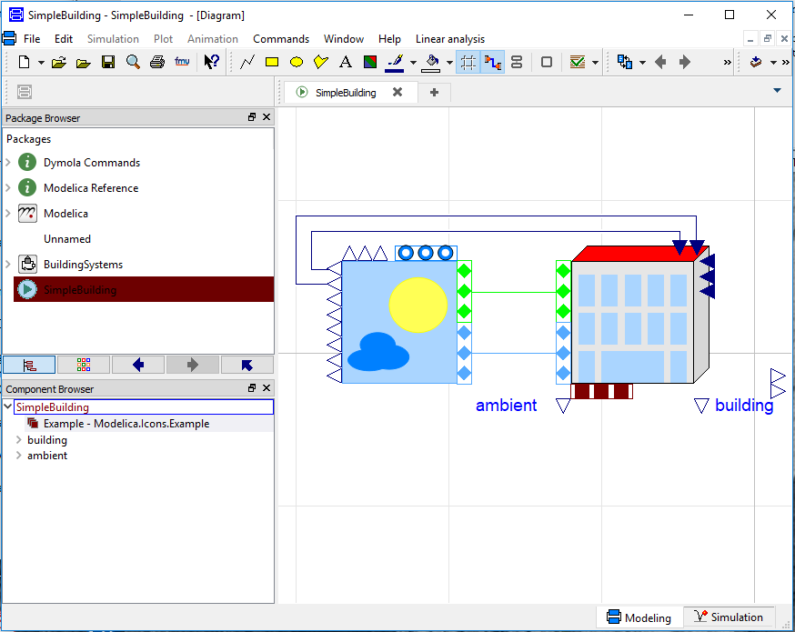
The simulation model, which consists of a building model and an ambient model

7. Next, connect the green connectors ambience.toSurfacePorts and building.toAmbienceSurfacePorts of the ambience and the building model. This enables the ambient model to deliver the boundary conditions for short-wave radiation from the sun and the long-wave radiation exchange with the sky.

8. The ambient model needs to know the number of surfaces of the building model which are in contact with the ambient air. For this purpose double-click on the ambient component and add this information to the parameter ambience.nSurfaces by clicking on the small arrow/triangle to the right of the text field and selecting Insert Component Reference: building -> extends BuildingSystems.Buildings.BaseClasses.BuildingTemplate -> nSurfacesAmbience.

9. Connect the output variable ambience.TAirRef and the input variable building.TAirAmb (ambient temperature at a reference height of 10 m) and also ambience.xAirRef and building.xAirAmb (ambient absolute moisture). Both variables are necessary for the calculation of the energy loss caused by the air exchange of the building. Your model should now look like Figure 2.

2.2. Define the building model parameters

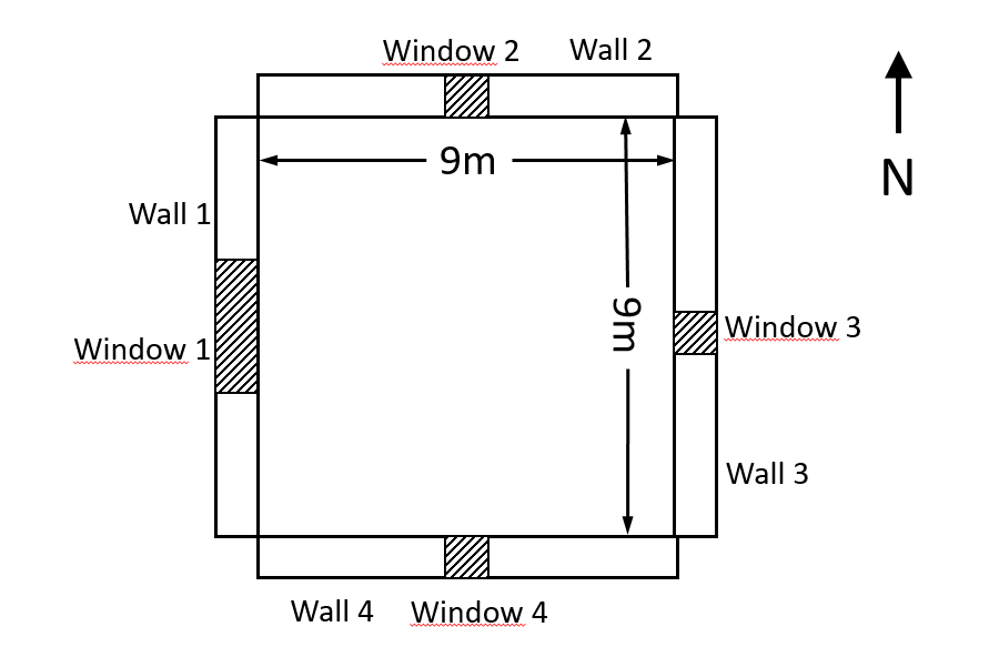
1. Define the building dimensions. The inner space of the example building is 9 m wide, 9 m long, and 3 m high. These dimensions are equal to the enclosed air space; the outer dimensions of the building model depend on the thickness of the selected wall, roof, and base plate constructions. Double-click on the building and fill in these values under Geometry within the tab General of the parameter dialog (see Fig. 3).

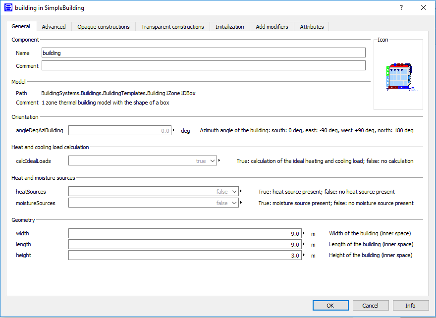
Definition of the geometry of the building model

2. Define the type of opaque construction in the building model component. For this purpose open the tab Opaque constructions (see Fig.4), and, in the group Exterior constructions, select

   • the type Outer wall construction for single-family house EnEV 2014 for all exterior walls (constructionWall1 to constructionWall4),

   • the type Roof construction for single-family house EnEV 2014 for the roof (constructionCeiling), and

   • the type BasePlate construction for single-family house EnEV 2014 for the base plate (constructionBottom).

   Set the parameters InteriorWalls and InteriorCeilings to “false” (group Interior constructions on the same tab), because, for this example, interior constructions will be neglected.

   It is worth noting that the walls and windows are numbered 1 = West, 2 = North, 3 = East, and 4 = South, as shown in Figure 5.

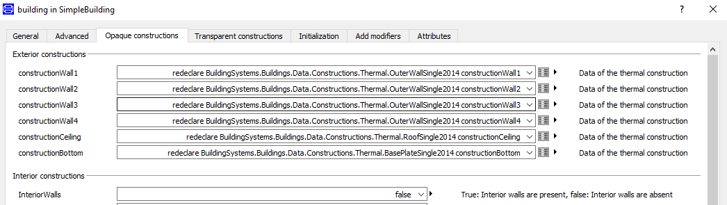
Definition of the opaque constructions

Cardinal directions as defined in Modelica

3. Define the type of transparent constructions in the building model. In the tab Transparent constructions (see Fig. 6), select the construction type Heat protection double glazing with UValGla=1.4W/(m2.K) and g=0.58 for all windows (window1 to window4) . Define the size of window1 to 3 m width by 1 m height and window2, window3, and window4 to 1 m width by 1 m height. Set the frame portion of all of the windows to 0.3.

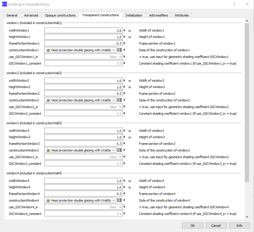
Definition of the transparent constructions

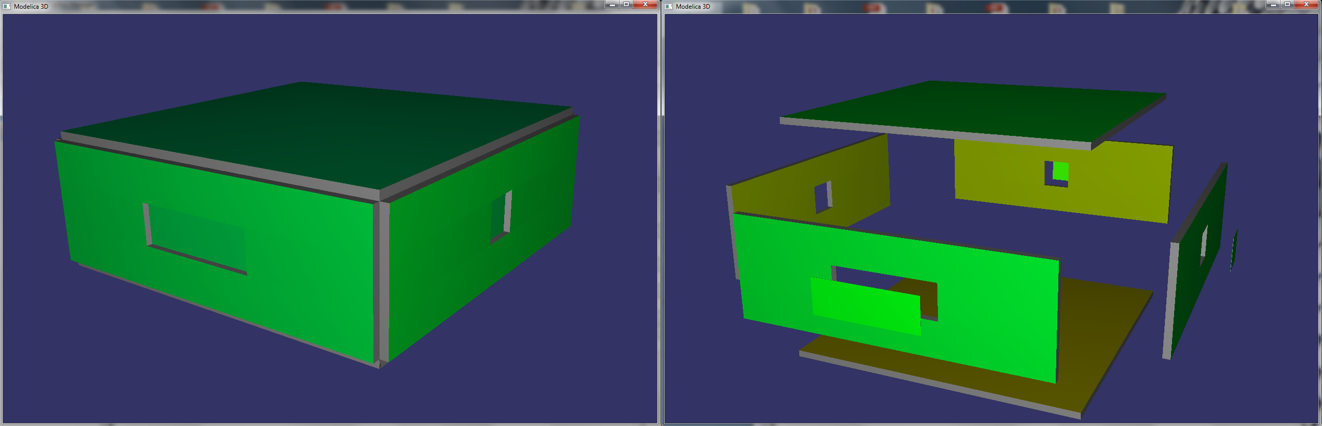
Left: Visualization of the building model with the color illustrating the surface temperatures of the building constructions. Right: Exploded visualization of the building model.

2.3. Set the boundary conditions of the building model

1. Define the set temperatures for heating and cooling and the air change rate. To define the set temperatures and the air change rate, find the MSL model class Modelica.Blocks.Sources.Constant in the package browser menu and drag and drop three instances of it into the system model. Rename them to TSetHeating, TSetCooling and airchange and parametrize them with 273.15 + 20.0 (20 degrees Celsius) 273.15 + 24.0 (24 degrees Celsius) and 0.5 (half an air change per hour) respectively. Connect the output of the three blocks with the corresponding input variables building.TSetHeating, building.TSetCooling and building.airchange on the upper right corner of the building model. For a smoother connection, you can right-click on the blocks and flip them horizontally.

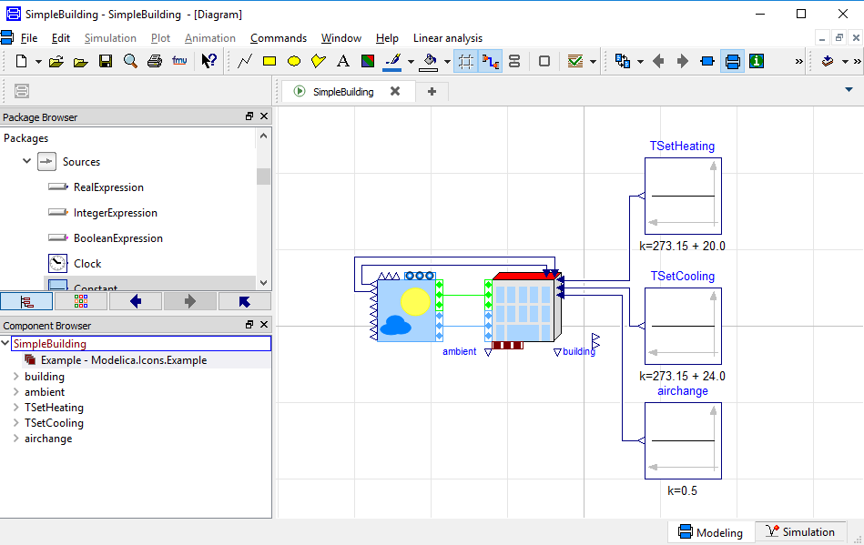
Completed system model with boundary condition (set temperatures, air change rate)

The Modelica code of the described example of this chapter can be found under

https://github.com/UdK-VPT/BuildingSystems/blob/master/BuildingSystems/Resources/Documentation/ExamplesUserGuide/SimpleBuilding.mo .

2.4. Simulate the system model

Now the model is 100 percent prepared for a simulation analysis. Simulate the model over a time period of one year. To do this, select the experiment SimpleBuilding in the package browser of Dymola and switch to the simulation mode.

1. Open the Simulation Setup dialog and fill in 31536000 (3600 seconds/hour x 24 hours/day x 365 days/year = 31536000 seconds) into the Stop time entry field and perform the simulation experiment.

2. Study the simulation results: the next two diagrams (Fig. 10 and 11) show the main important temperatures (outside and inside air temperature, operative temperature) and the ideal heating and cooling power for the building, which guarantees that the indoor air temperature remain in the desired area between 20 and 24 degrees Celsius.

The first diagram illustrates that the indoor air temperature and the operative temperature (the mean value of the indoor air temperature and the mean surface temperature within the zone) are close together. The reason is the insulated construction of the walls, the ceiling and the base plate in accordance with the current German energy code (EnEV 2014). The indoor air temperature only reaches maximum values of 24 degrees Celsius during some summer days.

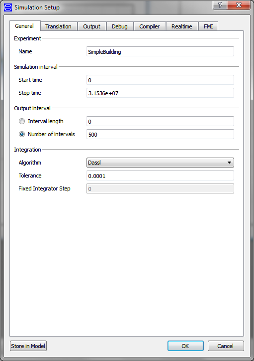
Simulation set-up window

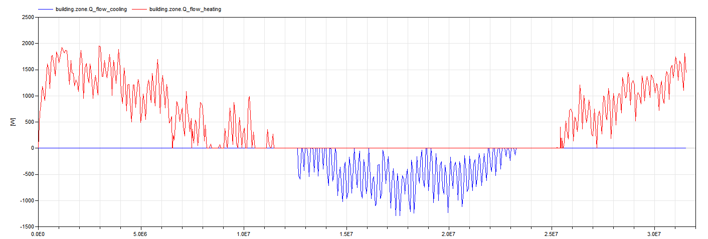
In the location Berlin, close to 100 percent of the thermal energy demand is made up of heating energy. A small amount of cooling energy is only needed during some of the hot summer days.

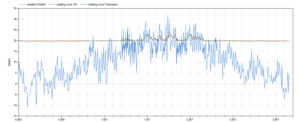
Air temperature, operative temperature and ambient air temperature during the yearly simulation (location Berlin, Germany)

2.5. Change the climate location

In the next step, change the location of the building to study the impact of a hot and dry climate on the thermal energy demand of the building model in comparison to the moderate climate of Berlin. Double-click on the ambient component and change the parameter weatherDataFile within the component to Iran_Hashtgerd_Meteonorm_NetCDF. Hashtgerd is a city in northern Iran, 100 km west of Tehran.

The outside temperature in Hashtgerd is close to 40 degrees Celsius during the summer (compare to Berlin 32 degrees Celsius). This leads to a significant cooling demand in summer, but there is still a relevant heating demand in winter.

Thermal energy demand for heating and cooling during the yearly simulation (location Berlin, Germany)

Air temperature, operative temperature and ambient air temperature during the yearly simulation (location Hashtgerd, Iran)

Thermal energy demand for heating and cooling during the yearly simulation (location Hashtgerd, Iran)